lm()
The lm() function fits a linear model to data.
 Example 1:

Example 1:
# fits an empty model
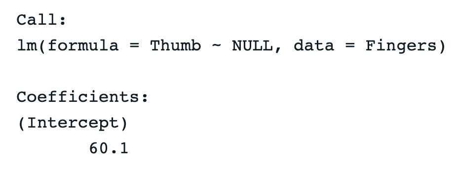
lm(Thumb ~ NULL, data = Fingers)
Example of output from running the code above:

 Example 2:

Example 2:
# fits a model with one explanatory variable
lm(Thumb ~ Gender, data = Fingers)
Example of output from running the code above:
Related Articles
gf_lm()
The gf_lm() function overlays the best-fitting regression line on a scatter plot when chained onto gf_point(). Example: # adds a regression line gf_point(Thumb ~ Height, data = Fingers) %>% gf_lm( color = "orange", size = 2 )predict()
The predict() function will generate the prediction(s) from a model. Example 1: # Calculate the predictions from the Gender model of Thumb # Use the lm() function to specify the model predict(lm(Thumb ~ Gender, data = Fingers)) # Alt: Save the model ...supernova()
The supernova() function will compute an analysis of variance (ANOVA) for a model, and present the statistics in a modified ANOVA table, that includes: - sums of squares (SS) - degrees of freedom (df) - mean squares (MS) - proportional reduction in ...anova()
The anova() function will compute an analysis of variance (ANOVA) for a model, and present the statistics in an ANOVA table, that includes: - sums of squares (Sum Sq) - degrees of freedom (Df) - mean squares (Mean Sq) - F values - p-values (Pr(>F)) ...confint()
The confint() function computes confidence intervals (based on the t-distribution) for one or more parameters in a fitted model. The default confidence level is 95%. To adjust the confidence level, use the "level = " argument. Example 1: You can use ...